Deep Learning
Explore the core concepts of deep learning, including how artificial neural networks mimic brain neurons, the role of activation functions in learning nonlinear relationships, and types of network architectures. Understand how models train using backward propagation to improve predictions and when to consider deep learning for complex problems.
We'll cover the following...
Introduction
For decades researchers have been trying to deconstruct the inner workings of our incredible and fascinating brains, hoping to learn to infuse a brain-like intelligence into machines. For example, when we were toddlers, we did not learn to recognize objects by learning their distinctive features. A child learns to call a cat “a cat” and a dog “a dog” by being exposed to the same example many times and by being corrected for the wrong guesses. This extremely active, “inspired from the brain” field of artificial computer intelligence is called deep learning. The corresponding programming paradigm, which allows computers to learn from data, is called artificial neural networks (ANN).
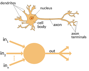
Just like a biological neuron has dendrites to receive signals, a cell body to process them, and an axon to output the signals to other neurons, the artificial neuron (also referred as a perceptron) has a number of input channels, a processing unit, and an output channel that can send signals to multiple other nodes.
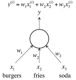
Each input (x0, x1, x2) to the neuron has an associated weight (w0, w1, w2), which is assigned on the basis of its relative importance to other inputs. Each of the inputs is multiplied by its weight, and then the processing unit applies a transformation function f, called the activation function, to the weighted sum of its inputs, as shown in the figure below.

The ANN additionally takes another input 1 with weight b (called bias, shown in the blue circle). The activation function f, used to compute the final output Y (where Y = f(x0.w0+x1.w1+x2.w2 + b)), needs to be a nonlinear function. This is because ANN needs to learn complex relationships. We will see what this exactly means in a while.
Before moving on, let’s break down this whole process in steps and visualize it with an animation:

- Each input is multiplied by its weight.
- The weighted inputs are summed to a single number, and a bias is added.
- The output from step two is passed through a nonlinear function to produce the final output.
Activation functions
Why do we need activation functions?
For example, if we simply want to estimate the cost of a meal, we could use a neuron based on a linear function f(z) = wx + b. Using (z) = z and weights equal to the price of each item. The linear neuron would take in the number of burgers, fries, and sodas and output the price of the meal.
The above kind of linear neuron is very easy for computation. However, by just having an interconnected set of linear neurons, we won’t be able to learn complex relationships. Taking multiple linear functions and combining them still gives us a linear function, and we could represent the whole network by a simple matrix transformation.
Real-world data is mostly non-linear, so this is where the activation functions come for help. Activation functions introduce non-linearity into the output of a neuron, and this ensures that we can learn more complex functions by approximating every non-linear function as a linear combination of a large number of non-linear functions.
Also, activation functions help us to limit the output to a certain finite value.
The activation function (non-linearity) simply needs to take a number as input and apply a mathematical operation on it. There is a rich variety of activation functions but the most commonly used ones are Sigmoid, Tanh, and ReLU.
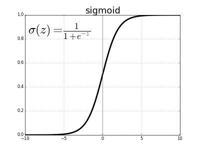
For example, the Sigmoid activation function takes a real-valued input and outputs a number between 1 and 0, as shown in the figure below. Intuitively, when the input is very small, the output of the neuron is very close to 0. When the input is very large, the output of the neuron is close to 1. In between the two extremes, it is S-shaped.
Neural network architecture and types
The components of a neural network:
- Input layer: These nodes are responsible for passing the input information to the hidden layer without performing any computations. (A set of nodes is called a layer.)
- Hidden layer (not an input or an output): These are the nodes where all the computations occur and they transfer information from the input nodes to the output nodes. While a network can only have a single input and output layer, there can be multiple (or no) hidden layers.
- Output layer: This is where the final output is calculated (using activation functions).
- Weights: Each of the connections between nodes has an associated weight.

So far, we’ve looked at models where the output from one layer is used as input to the next layer. Such networks are called feedforward networks. There are no loops in the network, meaning information is always transferred forward and never fed back. Having loops means ending up with the case where the input function f(z) is dependent on the output. The models where we have such feedback loops are called recurrent neural networks (RNNs). To allow for backward propagation (information flowing in the backward direction for learning and updating weights), RNNs have internal memory. They are very handy for tasks where we are dealing with sequences, like for understanding speech or texts.
Feedforward networks can be split again into two main categories:
- Single layer perceptron: These are the simplest form of NNs as they have no hidden layers (like in the initial examples/figures).
- Multi layer perceptron: When we have one or more hidden layers, these ones are used for practical purposes and not just for theoretical explanations.
How does the model learn?
One of the most frequently used methods for training ANNs is called backward propagation or “learning from mistakes.” As we have seen, for any given set of inputs, the output of an ANN is dependent on the weights of the edges connecting the nodes in the network. Therefore, we want to learn the values for the weights to minimize the final error; the weights that minimize the errors we make on the training examples.
Without “Mathy” details, this is essentially what happens: Initially, all the weights are assigned random values. For every input sample, we calculate the final output and the prediction error. Then we propagate this error back to the previous layer, where it is used to adjust weights. Once all the layers are done adjusting weights, we use the new weights to calculate the new prediction error. This process of adjusting weights based on the final error is repeated until we have achieved an error below the desired threshold.
Concluding remarks
Deep learning solutions are ideal for tackling large and highly complex machine learning tasks, such as recommending the best videos to watch to hundreds of millions of users every day, like YouTube, and Netflix, or for powering speech recognition services, like Alexa and Cortana. Also, deep learning algorithms are black-box algorithms, so when starting a new machine learning project, you should not jump to them just because deep learning solutions sound cooler. If possible, start simple.